
These are separate Containerlab labs I keep in Forgejo to practice the parts of a network that are easy to talk about and much more useful to see fail. Each lab has its own topology, configuration, addressing, lifecycle commands, and verification. That separation matters. I can take down a link in the EVPN lab without disturbing the route-reflector lab or the CIN transport model.
The common theme is evidence. A container running is not proof that a network works. Each exercise starts with control-plane state, follows the selected route or forwarding state, and ends with an endpoint test or a packet capture. That is the same order I want to use when troubleshooting a real issue.
Seeing the topology live
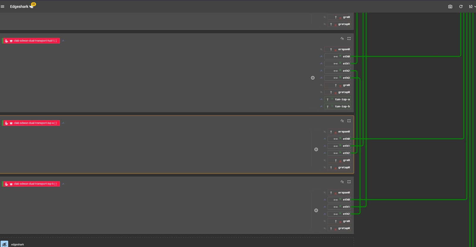
The static diagrams below explain the intent of each exercise. EdgeShark adds the live view: it shows the containers and links that actually exist on the Containerlab host. That is useful when moving from a topology file to troubleshooting, because the operator can see the running layout before selecting an interface for a packet capture.
How the labs are built
The direct Containerlab labs use pinned FRRouting and Alpine images. The topology, daemon configuration, setup steps, and verification script live together in the same lab directory. The larger fabric uses netlab to generate its Containerlab topology, device configuration, inventory, addressing data, and validation tests from one topology definition.
The labs are deliberately scoped. Each one has a distinct Containerlab name and management network, and teardown commands identify one topology file instead of using broad Docker or Containerlab cleanup. That lets more than one practice environment exist on the host without one lab quietly replacing another.
Route reflection: learn the control plane before adding an overlay
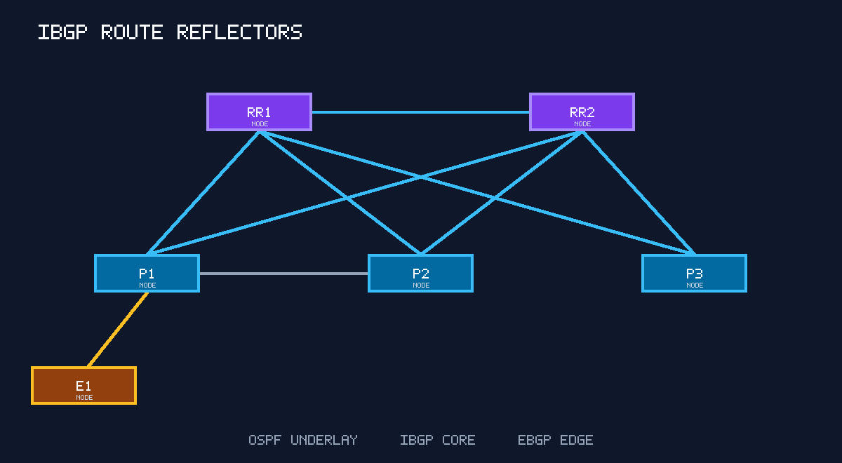
The route-reflector lab is the basic BGP exercise. It has two route reflectors, three iBGP clients, an OSPF underlay, and an eBGP edge. OSPF carries reachability between router loopbacks. The BGP sessions use those loopbacks, which separates physical link reachability from the overlay peerings that depend on it.
Route reflection solves the iBGP full-mesh problem. Instead of every client peering directly with every other client, each client peers with both reflectors. The reflectors distribute eligible routes while BGP attributes such as originator ID and cluster list prevent reflected routes from looping indefinitely.
This is a good place to watch a route move through the control plane. First, confirm the OSPF neighbors and loopback routes. Next, check both iBGP sessions. Then inspect the BGP entry for the external prefix, including its next hop and community, before checking whether it was installed in the routing table. If a route is missing, that sequence narrows the fault to transport, session state, policy, or route installation instead of treating BGP as one black box.
The eBGP edge also makes policy work visible. The lab advertises an external prefix with a community, so route filtering, local preference, and path selection can be practiced without needing a second physical network.
Why enterprises use route reflectors
iBGP has a scaling problem. In a full mesh, every router needs a session to every other router. That is manageable for a handful of routers, but the number of sessions grows quickly as the network grows. Route reflectors reduce that session count by giving client routers a small, predictable set of peers.
Enterprises and service providers use this pattern when they need one BGP domain across many routers, sites, or data-center devices. The route reflectors are usually chosen for stability and reachability rather than because they forward user traffic. Keeping them out of the normal data path means a forwarding problem and a control-plane problem are easier to distinguish.
The tradeoff is that the reflector design becomes part of the architecture. Clients need redundant reflectors, reflector placement affects route visibility, and policy needs to be understood before it is pushed broadly. A route reflector is not a shortcut around BGP design. It is a way to make that design operate at a larger scale.
EVPN and VXLAN: separate the underlay, control plane, and data plane
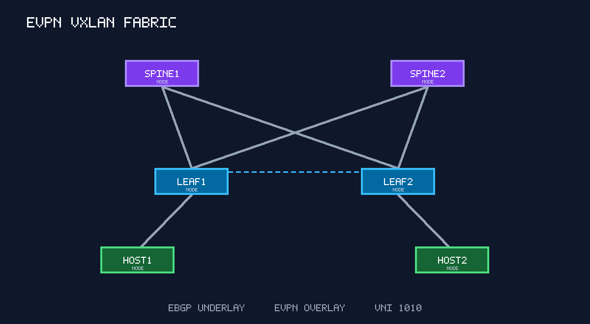
The EVPN lab is a two-spine, two-leaf FRR fabric. The spines are transit and control-plane nodes. The leaves are VTEPs and connect to one endpoint each. The fabric has an eBGP underlay, loopback-based EVPN sessions, and one stretched Layer 2 segment using VNI 1010.
The underlay has one job: carry IP traffic between the VTEP loopbacks. It should work before EVPN is considered. The leaves then use BGP EVPN to exchange the information needed to build the overlay. VXLAN carries the endpoint frames between the VTEPs across the routed fabric. Keeping those layers distinct is what makes a failure understandable.
The verification script follows that dependency order. It checks the underlay BGP sessions, tests VTEP reachability, checks the EVPN sessions and Type 3 routes, checks the VXLAN interface and bridge forwarding database, and finally pings between the two endpoint containers. A passing endpoint ping by itself is useful, but it does not explain which part made it work. The intermediate checks do.
The failure drills use the same structure. Shutting one leaf uplink should leave a second path to the remote VTEP. Stopping one spine should show how the remaining transport path carries the traffic. Removing EVPN configuration from one leaf should change the advertised routes and flood-list state. An MTU mismatch demonstrates why an apparently healthy IP path can still fail after VXLAN encapsulation adds overhead.
Why enterprises use EVPN and VXLAN
Traditional Layer 2 designs often depend on large broadcast domains and flood-and-learn behavior. That can work, but it becomes harder to extend across a large data center without making the failure domain larger too. EVPN uses BGP to distribute endpoint and segment information. VXLAN carries the tenant traffic across an IP fabric, which lets the physical network stay routed and multipathed.
This is attractive when an organization needs active paths across a leaf-spine fabric, workload mobility, tenant segmentation, or a repeatable way to add racks without redesigning the whole network. The leaf switches are the point where endpoint traffic enters the fabric. The spines provide transport between leaves. That role separation is why losing one spine should reduce capacity, not isolate a leaf.
EVPN is not automatically the right answer. Small environments may be better served by simple VLANs and routed links. A fabric also needs clear decisions about tenant VRFs, gateways, route advertisement, multicast or replication behavior, and operational ownership. The lab keeps the first stage to one Layer 2 VNI so those dependencies can be learned before adding distributed gateways and Layer 3 VNIs.
CIN and Remote-PHY transport: model the IP transport, not the whole cable plant
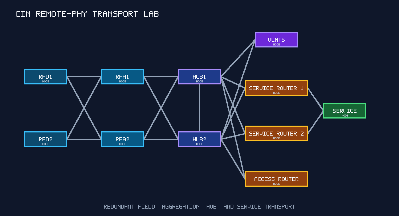
The CIN and Remote-PHY lab is intentionally narrower than the name suggests. It models the IP transport that carries distributed-access functions. It does not emulate DOCSIS RF, modem registration, RPD control protocols, or a vendor vCMTS.
There are two field RPD roles, two RPA aggregation roles, and two CIN hub roles. The hubs have separate redundant branches toward a vCMTS role, two service-router roles, an access-router role, and a generic service endpoint. The diagram is arranged to make one important design point clear: the hub-attached roles are parallel dual-homed branches. They are not one serial CMTS to Access Router to Service Router service path.
The current lab uses OSPF area 0 as a simple, observable baseline. It supports redundant paths, ECMP, failover, DSCP observation, and fault-isolation exercises. For example, taking down one RPD transport leg should leave the other path available. The correct proof is not just an interface state. It is the changed neighbor and route state plus a successful flow to the service endpoint.
The real transport design uses IS-IS and iBGP over routed loopbacks. That work is being kept separate from the baseline instead of being guessed into the topology. The model also keeps management and routed transport distinct. A generic Containerlab management interface is only a functional analogue, not evidence of a vendor management design.
Why a transport model matters in distributed access
Distributed-access cable architectures move functions that were once concentrated in a hub into field and virtualized roles. The transport network becomes more important because it carries multiple service-facing paths between those roles. Redundant aggregation and hub connectivity are used so one link or one device failure does not immediately remove every available path.
Whether an enterprise or operator uses this exact layout depends on its platform, geography, scale, vendor design, and service requirements. The lab is not trying to claim that every environment has the same RPA, hub, service-router, or access-router role. It is useful because it makes the transport questions concrete: where does routing terminate, which paths are redundant, what is a logical service branch, and what evidence proves the remaining path is carrying traffic.
The model keeps access-router behavior deliberately limited to what the transport exercise needs. A diagram can be useful without pretending that every label has been fully decoded. The operational focus stays on the interfaces, routing adjacencies, route tables, and reachability that can actually be tested.
Dual transport and the SD-WAN question
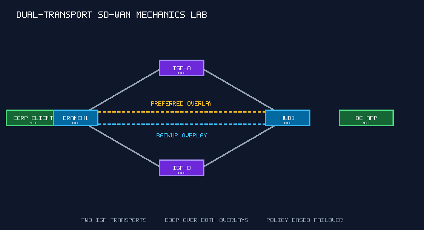
A separate lab models the core mechanics behind dual-transport SD-WAN. A branch and hub have two ISP paths, GRE overlays across both transports, eBGP over the overlays, and policy that prefers one path while retaining the other as a backup. The normal test is simple: remove the preferred overlay, confirm that its BGP session drops, confirm that the route moves to the backup tunnel, and prove that branch-to-data-center traffic still works.
Real SD-WAN platforms add controller-based policy, encrypted tunnels, application classification, path measurement, zero-touch provisioning, and centralized operations. They are useful when an organization has many sites, multiple transport types, and a need to apply consistent policy from one place. A small site with one or two straightforward WAN links may not need that control plane or its operational overhead.
The lab uses GRE because the encapsulation and failure domains are easy to inspect. GRE is not encrypted and is not being presented as a production security design. The point is to make the routing decision visible first. IPsec or WireGuard can be introduced later without changing the basic question of how the branch selects and fails over between transports.
The larger enterprise fabric
The enterprise-fabric project is the next step up in tooling and scale. It is a six-switch SR Linux design generated by netlab: two spine route reflectors, four leaves, OSPF underlay reachability, and iBGP over loopbacks. Every leaf originates a different prefix so route reflection and failure behavior are easy to inspect.
netlab generates the device configuration, Containerlab topology, Ansible inventory, addressing, and validation data from the source topology. That avoids hand-maintaining several copies of the same intent. The planned operations layer adds SSH and gNMI management, Ansible reachability checks, and Telegraf, InfluxDB, and Grafana for interface and BGP telemetry.
That fabric is source-ready, not presented as deployed. The current Containerlab VM has limited CPU and memory, so the full SR Linux and observability stack stays behind a capacity check. That is a deliberate constraint. A smaller lab that can be started, verified, and torn down predictably is more valuable than an oversized one that makes the host unreliable.
Automation and observability are part of the design
Automation is most useful after the network has a known-good baseline. In the larger fabric, netlab generates the initial configuration and inventory. Ansible can then validate reachability, collect state, and make bounded changes with a before and after check. That avoids trying to use automation as a substitute for understanding the network it is changing.
Observability follows the same rule. Interface counters, BGP neighbor state, and telemetry in Grafana are useful when they answer a specific question. They do not replace a routing-table check or an endpoint test. In a real enterprise, telemetry helps establish whether a problem is local to one interface, shared by a failure domain, or visible as a control-plane symptom. In the lab, it makes those relationships easier to learn.
Not every enterprise needs a full telemetry stack in every small environment. The value rises with device count, change rate, and the cost of being slow to diagnose a fault. The capacity gate on the SR Linux lab is an example of the same judgment. More tooling is only an improvement when the host and team can operate it reliably.
Why keep all of this?
The labs are not meant to replace production systems. They make protocol behavior visible before it matters in production. They give me a place to rehearse the troubleshooting sequence, test a policy change, capture traffic, and learn what healthy and degraded state actually look like.
When an exercise is finished, the useful result is not the diagram. It is the evidence: neighbor state, selected routes, EVPN routes, forwarding entries, endpoint traffic, packet captures, and a clear explanation for why the network behaved the way it did.